Deep Learning algorithms are being used more often to process remote sensing data. Data captured from satellite platforms requires reliable and generalized methods to periodically extract and analyse useful information. Environmental planners are becoming increasingly interested in applications, such as land cover mapping ranging from urban development to crop detection, to monitor climate change and wildfires.

In the summer of 2021, a catastrophic rain storm hit Europe and devastated properties. Major cities in Germany were severely affected, especially in Rhineland-Palatinate, the south of North Rhine-Westphalia, and parts of Bavaria. The floodwaters destroyed highways, houses and entire towns, tragically leaving hundreds of people dead, injured or missing. Rescue teams rely on a timely information product of flooded areas with a wide coverage, especially when a large area is affected.

Remote sensing is generally a convenient way to obtain near-real-time information and monitor the earth over a large area. However, satellites with optical imaging sensors, such as Landsat 8, suffer from a lack of data during rainfall events. This is due to the clouds and weather conditions that block spectral reflectance. Furthermore, the satellites usually take longer to orbit the earth, which delays the processing of the event.  On the other hand, radar-based sensors, such as Sentinel 1, use microwaves that can penetrate haze, light rain and clouds to illuminate the earth and measure the backscatter and travel time of the transmitted waves reflected by objects on the ground.

When applied to radar images, so-called Synthetic Aperture Radar (SAR) images, modern Deep Learning algorithms make it possible to improve flood detection. In the case of Sentinel 1, the raw data consists of polarized bands VV and VH.  We applied a data preparation workflow similar to the one described in [1]. We used the python library snappy of the SNAP API to perform data pre-processing.  The steps of data preparation are shown in Fig. 1.

First, we applied thermal noise removal and then calculated the calibration of physical units. Afterwards, we applied a speckle filter using Gamma Map with a window size of 3×3 pixels to reduce noise and artifacts. In order to eliminate different topographical distortions such as shadowing and layover effects we applied terrain correction using the parameter of “SRTM 1Sec HGT”, which allows us to obtain the precise geolocation information of each pixel in the image. Then we used upsampling to a spatial resolution of 30m with bilinear interpolation. Lastly, we converted the values of the backscatter into decibel using logarithmic scaling.

After completing the preprocessing step, we developed a Landsat-Water Classifier that uses Landsat 8 cloud free images. In order to train a model to predict water surfaces using a Landsat 8 image, it is important to first obtain training data that consists of pairs of input and label images. The input images are calibrated Landsat scenes conditioned by a constraint of 1% maximum cloud cover – since optical reflectance cannot penetrate clouds, which affects the quality of the training data. We have stacked 6 different Landsat bands as input images: blue, green, red, near-infrared and Short-wave Infrared 1 and 2. The label images consist of binary masks of water surfaces (water = 1 and non-water = 0). The National Forest Information System (NFIS) obtains the label data as a water class in the forest land cover for Canada 2015 Dataset. It was possible to obtain georeferenced data from different sources, because the reprojection of the images guarantees overlapping of both datasets and hence facilitates image registration.

 

The Landsat-Water Classifier is a semantic segmentation model that was trained on 12 different Canadian Landsat scenes in 2015. The model has a u-net architecture consisting of 5 convolution and deconvolution layers. We applied the binary cross entropy loss function, which uses the dice coefficient to evaluate accuracy, to train the model to classify water. The model has reached a total accuracy of 93% after learning for 40 epochs.

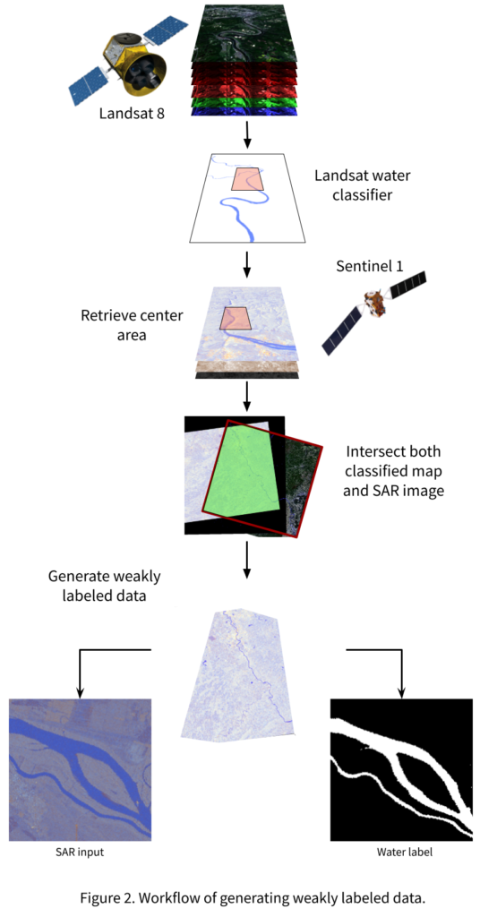
The label data for the SAR images were generated using the Landsat-Water Classifier while intersecting with SAR images. The idea of generating weakly labeled masks using a pre-trained model is based on the fact that the only available dataset of a specific period of  time that has low overlap with Sentinel 1 images was in the Canada 2015 scene. Fig. 2 describes the workflow of generating patches of pairs containing weakly labeled SAR images. The process is fully automated. It starts with defining the area of interest and the time window to search for training images. We use the EarthExplorer API with the maximum clouds cover of 1% constraints to collect Landsat 8 scenes. Then, using Landsat-Water Classifier, we can generate a full scene of water masks. We calculate a bounding box in the center of the Landsat scene. This we use as a parameter to retrieve Sentinel 1 scenes. We include this center area by means of the Sentinelsat [2]. We generated over 1000 image patches of 512×512 pixels. We ensured that the patches have a roughly balanced pixel ratio of water = 1 and non-water = 0.

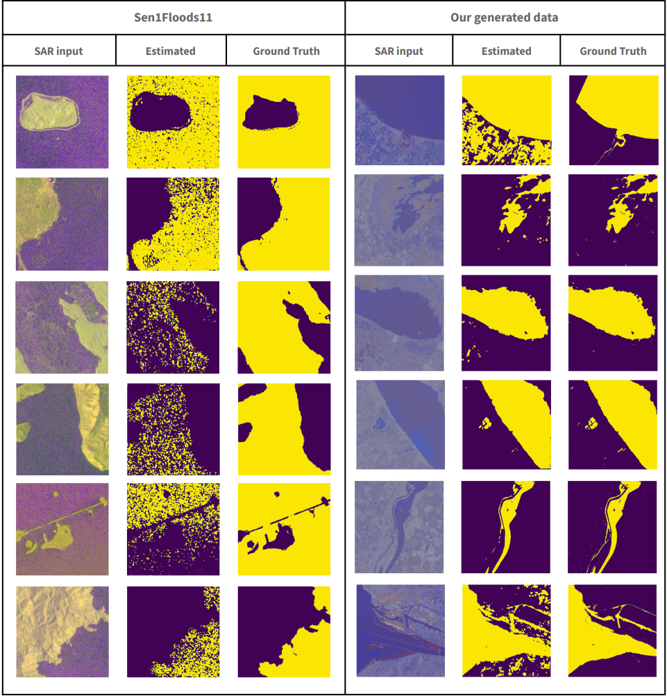
The dataset generated was used to train the Sentinel-Water Classifier that can predict permanent water surfaces from SAR images. For the model, we used a denser u-net architecture, namely, Unet++. The advantage of Unet++ is having more convolutional layers along the skip connections to embed more semantic features into the decoder. A weighted loss function consisting of binary cross-entropy and a dice coefficient loss weighted with 0.15 and 0.85 were used respectively. We applied 5-fold cross validation to evaluate the model and to assess the quality of the water masks. Previous work was done on the same subject and provided the publicly available dataset Sen1Floods11. We also tested our model for permanent water surfaces using SAR images on the Sen1Floods11 dataset’s external data.

Results

The model has a mean IoU of 0.46 to predict permanent water surfaces on unseen data generated and calibrated using our workflow, whereas it has a mean IoU 0.50 on the Sen1Floods11 external dataset. This can be due to the accuracy of the labels generated.

Conclusion

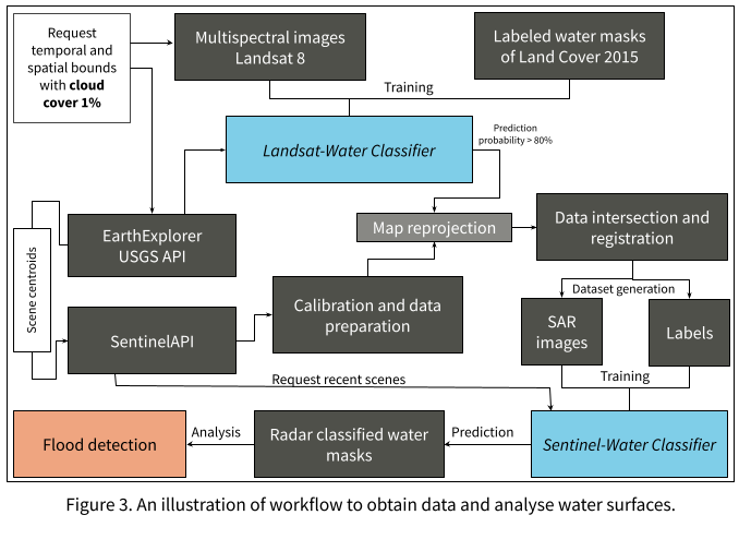
The proposed workflow, which is illustrated in Fig. 3, suggests a solution to provide labeled data of permanent water surfaces of SAR images. We then trained a model that discriminates between water surfaces and other objects. Eventually, we can use the model to analyze affected areas using different GIS applications. For instance, the difference between a scene recorded previous to a heavy rainfall event and one during or right after the event will lead to a flooding mask.

A possible drawback of our approach is the training of the Landsat Classifier in a different region (from a different project context) than the area of interest. However, quick cross-checks showed a very good alignment. A general limiting factor of EO data is the orbiting time of the satellite in correspondence with the event of interest. It is also possible to generate training data exclusively of flood events by adjusting the request area and timing. The pipeline is fully automated. This has the benefit of having a unique dataset of a climate event, which can be used in various applications.

The Sentinel 1 SAR images have the clear advantage of being far less weather dependent than the corresponding products based mainly on the visible spectrum. Ultimately, one can deploy this workflow in the cloud to be able to provide a near real time information product.

This work has partially been possible through the KI:STE project funded by the German Federal Ministry for the Environment, Nature Conservation and Nuclear Safety under grant agreement number 67KI2043.