This post will also be EGU Session ERE1.1 Display D924 at EGU2020: Sharing Geoscience Online. We will participate in the chat on Tuesday, May 5th from 8:30 to 10:15 to discuss our approach and findings. You can join the discussion on our parallel medium.com story.

Estimating fuel consumption of cars based on movement data and its sensitivity to car and movement specific properties

The transportation sector is responsible for approximately 20 percent of global CO2 emissions, most of which are produced by road traffic. Moreover, emissions are rising and are rising faster than in other sectors. Reducing these emissions is crucial to reaching the goals of the 2016 Paris agreement. Efficient reduction strategies and their monitoring rely on broad and exact data about passenger car fuel consumption and emissions.

To encourage people to drive eco-efficiently and to collect traffic data, 52°North initiated the open Citizen Science Platform enviroCar. Data from the vehicle’s on board diagnostics can be sent to the enviroCar Android App via an OBD-Bluetooth adapter and then anonymized and uploaded as open data to the enviroCar server. Fuel consumption – and thus emissions – are conventionally calculated from motor-specific data like mass-air-flow. One drawback of this approach is that users need to have an OBD adapter installed to get these specific data. An easier and broader use of the app is achieved if one calculates the energy consumption based on the movement data measured via GPS sensors in the mobile phone.

We present such a purely GPS-based approach and the means to assess the sensitivity of the resulting fuel consumption to vehicle parameters and the movement pattern. The vehicles and track patterns analyzed show a high degree of heterogeneity regarding size and weight of vehicles as well as speed, acceleration and road gradient. In total, we analyzed 51 tracks from the open enviroCar server covering 7600 km within 95 hours.

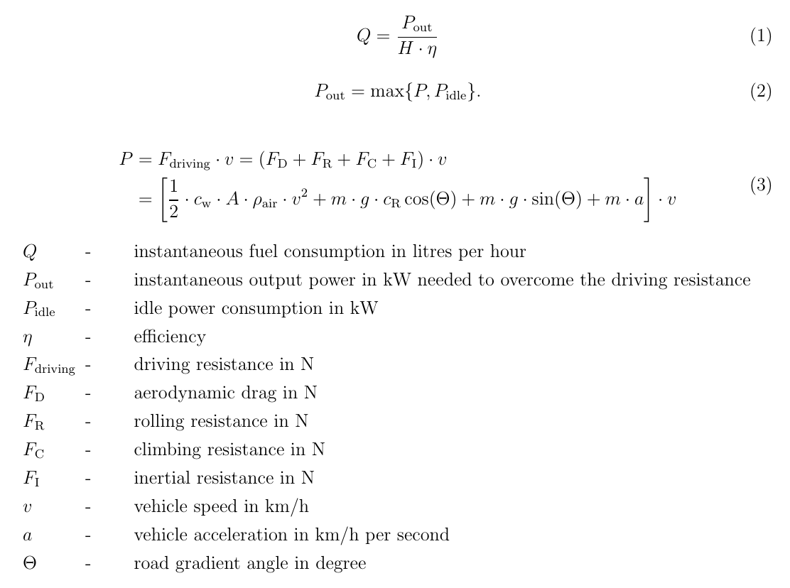
Instantaneous fuel consumption is load-based and calculated using Equations 1-3.

Whereas movement-related parameters like speed and acceleration are taken from the enviroCar data base, some additional parameters need to be taken from external sources (see Table 1). Parameters specific to a vehicle are constant for all cars, because these data are not yet included in the enviroCar platform. We will also discuss the resulting errors in the following paragraph. An important parameter is efficiency. It depends strongly on driving conditions. To take these variations into account, we linearly interpolate efficiency from 0.1 at −2000 N driving resistance to 0.4 at 2000 N or 0.43 for Diesel engines, respectively. This approach is based on the idea that the higher the driving resistance, the higher the engine load and thus the efficiency.

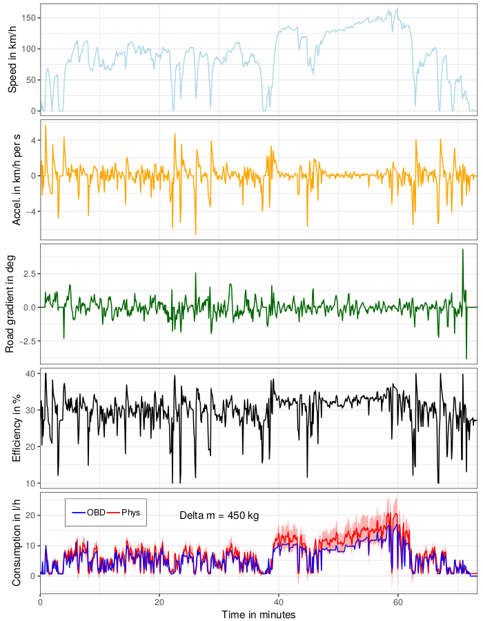
Figure 1 shows an example of movement patterns and fuel consumption calculated for a track collected with a Renault Clio. A speed of up to 160 km/h indicates that the car was driving on a highway, at least for part of the time. The lower image shows a comparison of calculated consumption with the consumption derived from the OBD. The values are similar except for the period between 40 and 60 minutes. We see discrepancies of about 5 l/h. The reasons for inaccuracies can be manifold. On the one hand, the calculation is simple and ignores, e.g. effects like wind or road conditions. On the other hand, the specified average vehicle-specific parameters diverge from the true values of the Renault Clio. For example, we can assume the true mass to be about 1050 kg. Using a linear error propagation, we calculated the resulting errors from a wrong mass, which is indicated by the red area. Obviously, this alone could explain the observed errors, however, it is only one possible factor. The influence of other factors can be estimated in the same fashion, which not only helps to understand the accuracy of load-based consumption models, but also indicates how car design and driving style influence fuel consumption.

In addition to the detailed analysis of specific tracks, we investigate the overall performance of 51 tracks using the consumption errors per 100 km. These are calculated using Equation 4

 

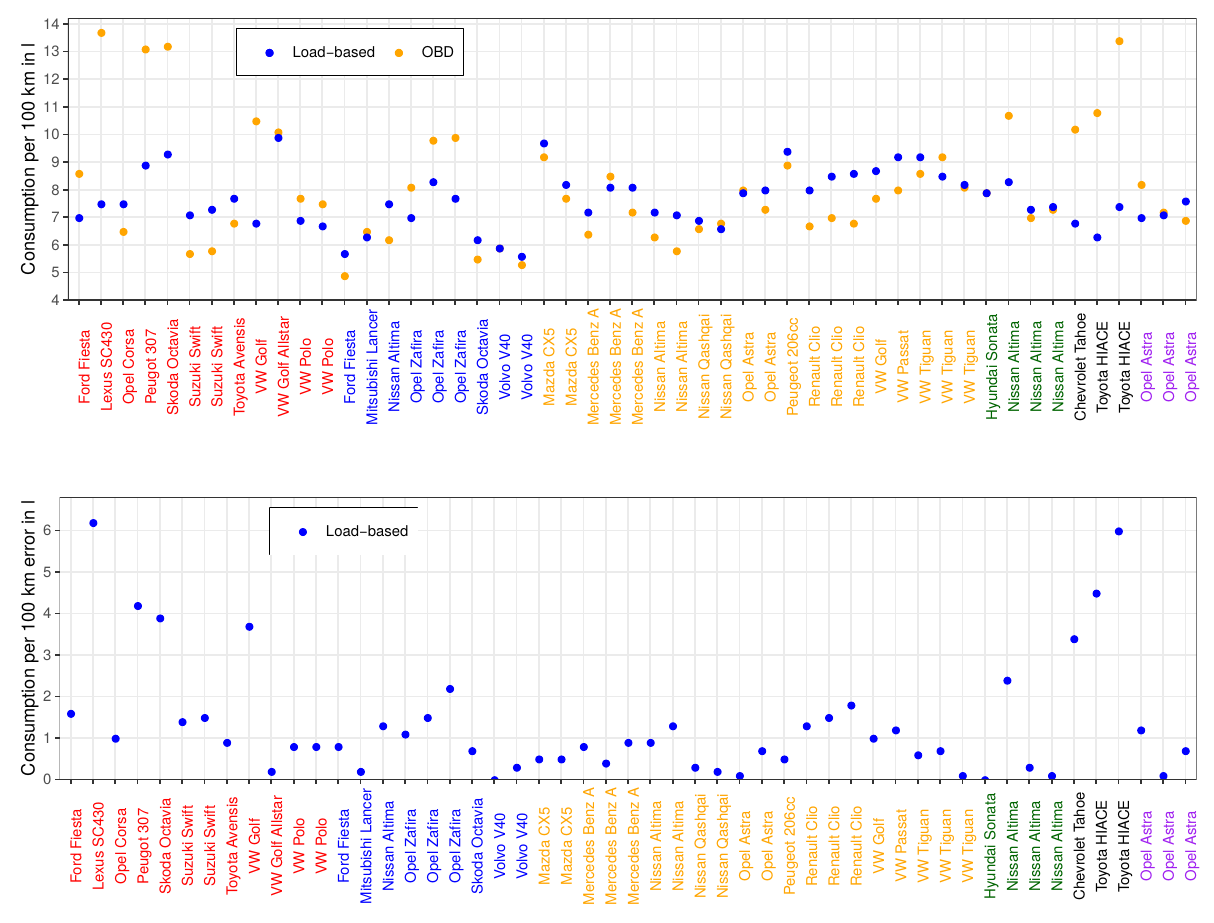
Figure 2 shows a comparison of the consumption per 100 km between the calculated and the OBD-derived values (top) and their differences (bottom). We can observe that for most tracks the differences are close to or below 1 l per 100 km. Errors tend to be larger for tracks with stop-and-go characteristics (red x labels). The large errors for the Toyota HIACE and the Chevrolet Tahoe (black x labels) are not surprising, because the true vehicle-specific parameters diverge largely from the values used in Table 1. Further, we note that the approach also provides reasonable results for Diesel cars (purple x labels). We only analyzed a few Diesel tracks, so this might limit the significance of our finding.

 

Despite the simplicity of our model, we are able to provide relatively precise values compared to consumption derived from the OBD with errors mostly close to or smaller than 1 l per 100 km. We can avoid some outliers by including true vehicle-specific parameters. Further improvements are needed for stop-and-go dominated tracks. One possibility would be to increase the temporal sampling rate. We might miss acceleration phases using the sampling of 5 s (with small exceptions), which leads to an underestimation of consumption. Although it has only been applied to cars with combustion engines, our approach is general and can also be applied to electric cars. In this case, we have to include a recuperation model and adapt the model to calculate efficiency.