Introduction

Hot spot analysis is a statistical tool to identify clusters in a dataset. In traffic management, identifying hot spots of ${\text{CO}}_2$ emissions might help to define measures for an overall reduction of emissions, e.g. by optimizing traffic light circuits in a hot spot. In the CITRAM project (Citizen Science for Traffic Management), citizens in three German cities (Chemnitz, Hamm and Krefeld) used the enviroCar App to collect extended floating car data (xFCD). The goal of the project was to understand how citizen science tools can contribute to improve traffic quality (e.g. efficient traffic flow, reduction of fuel consumption and emissions).

This article presents an exemplary hot spot analysis in the city of Hamm using data collected in calendar weeks 26 to 34 (June-August) in 2020. The data is based on a very small subset (about 900 trajectories) with a biased selection of drivers (mainly employees driving staff cars) during typical working hours. As a result, the following analysis does not necessarily represent the actual traffic situation in Hamm, but discusses the general insights that a hot spot analysis can generate.

Methodology

Getis Ord statistics

Spatial association is often analyzed using G statistics [1, 2, 3]. We first divide the area of interest into $n$ regions/features (e.g. points, lines or polygons) that are attributed with a specific value $x$, in our case ${\text{CO}}_2$ emissions. To identify a cluster, it is important to consider not only the value of a feature itself, but also the values of neighboring features. The local G index measures the local (weighted) mean value for each feature $i$ and is defined as follows.

$$\begin{array}{}\text{(1)}& G^{\ast }(i)=\frac{\sum _{j=1}^n{w}_{ij}{x}_j}{\sum _{j=1}^n{x}_j}\end{array}$$

where the star (${}^{\ast }$) implies that the focus feature $i$ itself is included in the index calculation. The weights $w_{ij}$ typically depends on the distance $d_{ij}$ between the features $i$ and $j$.

Under Gaussianity assumptions, $Z$-values are calculated for each feature $i$:

$$\begin{array}{}\text{(2)}& Z(i)=\frac{G^{\ast }(i)-E[G^{\ast }(i)]}{\sqrt{\mathrm{Var}{G}^{\ast }(i)}}\end{array}$$

A significantly large $Z$-value implies that large values are within the neighborhood of a feature. Such a feature is called hot spot. In contrast, if the $Z$-value is significantly small, the feature is called cold spot. For non-significant features the term grey spot has emerged. In general, we could use a more fine grained discretization of the classifications (e.g. based on regular quantiles).

Analysis steps

We used Jupyter Notebooks and the Python libraries envirocar-py, pandas, geopandas, numpy, pysal (esda, libpysal) to do the analysis and applied the following steps to obtain hot spot maps.

1. Read raw xFCD; extract coordinates, ${\text{CO}}_2$ emissions in kg/h and vehicle speed in km/h; optionally normalize ${\text{CO}}_2$ emissions by vehicle speed to emissions in kg/km
2. Remove outliers
3. Aggregate ${\text{CO}}_2$ emissions on equidistant grid with 30 m spacing
4. Calculate mean values of ${\text{CO}}_2$ emissions for each grid cell
5. Calculate row-standardized binary weights with a fixed distance band of 300 m (10 cells)
6. Calculate $G^{\ast }$ statistics for each feature (i.e. grid cell)
7. Under Gaussianity assumptions, define cells that are within the upper/lower 10 % of all $Z$-values as hot spot or cold spot, respectively

Results

In this section, we present one hot spot map for the original ${\text{CO}}_2$ emissions in kg/h and another map for ${\text{CO}}_2$ emissions normalized by vehicle speed in kg/km. We stress again that the data we use does not represent the statistical population, but only a scattered subset of the traffic in the corresponding time window of nine weeks. As a consequence, the results may suffer from a bias caused by the specific vehicle types, driving styles and traffic conditions.

Figure 1 shows a hot spot map for the original ${\text{CO}}_2$ emissions. Generally, hot spots tend to be present at street segments where cars can drive at high speeds, as instantaneous emissions correlate with speed in a physical sense. We expect acceleration and road gradient to influence the clustering as well.

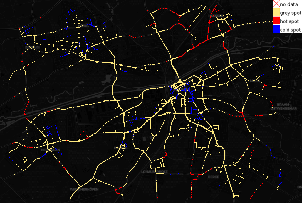
Cars might emit less ${\text{CO}}_2$ per hour when driving slowly; however, they also cover a smaller distance compared to a car driving at higher speed. To compensate for this effect and to gain a different view on the data set, we normalize ${\text{CO}}_2$ emissions by speed and recalculate the hot spot map (Figure 2). Some of the hot spots turned into cold spots and vice versa. However, many new hot and cold spots appeared. Cold spots generally seem to occur at street segments where we expect traffic to flow freely, i.e. outside the city center and between crossings. Hot spots are present where we assume there is stop-and-go traffic, i.e. at parking areas, crossings and in residential areas (presumably due to parking maneuvers).

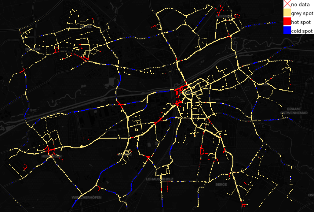
The representation of the data strongly influences the detection of hot and cold spots as you can see from Figure 1 (based on emissions in kg/h) and Figure 2 (based on emissions in kg/km). There are also various ways to tune and tweak the hot spot analysis: e.g. which metric $d$ is used and how do the weights $w_{ij}$ depend on the distances. Hence, one must execute and interpret any hot spot analysis with care and tailor it to the question at hand. A useful approach might be to filter the data apriori e.g. based on the street type, as hot and cold spots take into account the entire sample. If the focus of a traffic engineering project is on the comparison of emissions of major axes running through a city, the values collected along the minor roads will distort the distribution and hence the identification of the relevant locations. As a result, a hot spot analysis on heterogeneously sampled data might just identify the different extremes of the data collection and not the desired extremes of the sampled phenomenon.

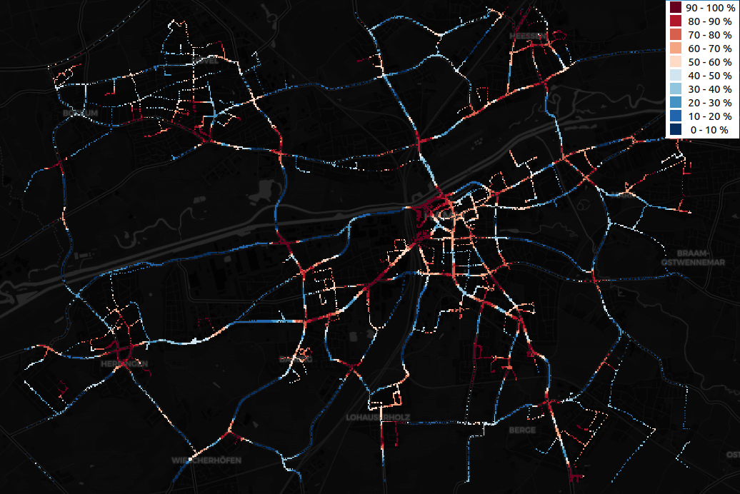
Another shortcoming might be the strict discretization in merely cold spots, grey spots and hot spots. The transition between these might also shed some light on the underlying features. As an example (Figure 3), we grouped the $Z$-values based on a series of quantiles. The original hot spots and cold spots are preserved, but the grey spots are further detailed and one gets a better overall view on the data and its distribution over the city.

Conclusion

We used xFCD from the enviroCar platform to perform a hot spot analysis of ${\text{CO}}_2$ emissions using open source Python tools. In combination with expert knowledge from those responsible for monitoring local traffic, e.g. employees of the city or traffic engineers, the results obtained can help understand and improve traffic quality.

The analysis performed represents an exploratory view on the data and can reveal general patterns. In order to answer specific questions, we need to adapt the algorithm, e.g. by performing the analysis on specific street segments or selecting specific time windows.

The CITRAM project is funded by the German Federal Ministry of Transport and Digital Infrastructure within the mFund framework under FKZ 19F2068.

Authors: Martin Pontius, Benedikt Gräler, Albert Remke

References

[1] Getis, A., & Ord, J. K. (1992). The analysis of spatial association by use of distance statistics.

[2] Ord, J. K., & Getis, A. (1995). Local spatial autocorrelation statistics: distributional issues and an application. Geographical analysis, 27(4), 286-306.

[3] Anselin, L. (1995). Local indicators of spatial association—LISA. Geographical analysis, 27(2), 93-115.